Quick start guide
I/O Options
The most simple code lines to use RADWave functions is summarised below
import RADWave as rwave

wa = rwave.waveAnalysis(altimeterURL='../dataset/IMOSURLs.txt', bbox=[152.0,155.0,-36.0,-34.0],
                stime=[1985,1,1], etime=[2018,12,31])
wa.processAltimeterData(altimeter_pick='all', saveCSV = 'altimeterData.csv')
wa.visualiseData(title="Altimeter data tracks", extent=[149.,158.,-38.,-32.],
               addcity=['Sydney', 151.2093, -33.8688], markersize=40, zoom=8,
               fsize=(8, 7), fsave='altimeterdata')
timeseries = wa.generateTimeSeries()
wa.plotTimeSeries(time=[1995,2016], series='H', fsize=(12, 5), fsave='seriesH')
wh_all = wa.computeSeasonalCharacteristics(series='wh', time=[1998,2018], lonlat=None, fsave='whall', plot=True)
Getting altimeter values from data providers
As previously mentioned, RADWave capabilities are illustrated using the Australian Ocean Data Network portal [AODN]. The altimeter dataset are available from the portal by searching for the following data collection:
IMOS-SRS Surface Waves Sub-Facility - altimeter wave/wind data
This global dataset has been compiled and extensively calibrated by [Ribal2019] and was regularly updated using altimeter data from 1985 to present. It can be downloaded in 1° x 1° URL files.
Note
The video below illustrates how to select both a spatial bounding box and a temporal extent from the portal and how to export the file containing the List of URLs used for wave analysis. This TXT file contains a list of NETCDF files for each available satellites.
Important
RADWave uses the file containing the list of URLs to query via THREDDS the remote data. This operation can take several minutes and when looking at a large region it is recommended to divide the analyse in smaller regions and download a series of URLs text file instead of the entire domain directly.
A series of URLs text files is provided with the notebook examples.
Loading altimeter parameters
Once the list of NETCDF data file has been saved on disk, you will be able to load it by initialising RADWave main Python class called waveAnalysis.
For a detail overview of the options available in this class, the user is invited to look at the waveAnalysis API.
import RADWave as rwave

wa = rwave.waveAnalysis(altimeterURL='../dataset/IMOSURLs.txt', bbox=[152.0,155.0,-36.0,-34.0],
                        stime=[1985,1,1], etime=[2018,12,31])
Note
In cases where one want to query altimeter data along a specific path such as a cyclone track, it will be necessary to provide a second file with the recorded track geographical coordinates and associated time. The file will be a CSV file with in the header the following keyword names lon, lat & datetime. An example of such a file is provided with the notebooks based on dataset exported from the Bureau of Meteorology (BOM). In such cases, the call to waveAnalysis will take the form:
import RADWave as rwave

wa = rwave.waveAnalysis(altimeterURL='../dataset/IMOS_YASI_east.txt', bbox=[170, 175, -17, -12],
                          stime=[2011,1,27], etime=[2011,2,4], cycloneCSV='../dataset/2010-YASI.csv')
After class initialisation querying the actual dataset is realised by calling the processAltimeterData function (option available in the processAltimeterData API)
wa.processAltimeterData(altimeter_pick='all', saveCSV = 'altimeterData.csv')
The function can take some times to execute depending on the number of NETCDF files to load and the size of the dataset to query.
Note
This function relies mostly on Pandas (library) and writes the processed dataset to file that can be later used to access more efficiently altimeter information.
In case where the processAltimeterData function has already been executed, one can load directly the processed data from the created CSV file in a more efficient way by running the readAltimeterData function as follow:
wa.readAltimeterData(saveCSV = 'altimeterData.csv')
Computing wave regime
To perform wave analysis and compute the wave parameters discussed in the documentation, two additional functions are available:
generateTimeSeriessee the generateTimeSeries API for the available options. This function computes time series of wave characteristics from significant wave height \(H_{s}\) and wind speed \(U_{10}\). It computes the both instantaneous and monthly wave variables. The classwaveAnalysisstores a Pandas dataframe (calledtimeseries) of computed wave parameters that can be subsequently used for further analysis. The following wave parameters can be plotted with this function:Hfor wave height,Tfor wave period,Pfor wave power,Efor wave energy, andCgfor wave group velocity.close2Tracksee the close2Track API for the available options. This function can be used when analysing cyclone tracks and finds the closest processed altimeter geographical locations that have been recorded in the database based on a KDTree search. As for the previous function, this one stores a Pandas dataframe (calledcyclone_data) of closest wave data that can be subsequently used for further analysis.
timeseries = wa.generateTimeSeries()
track = wa.close2Track(radius=2.,dtmax=6.)
Outputs
We provide several default plotting functionalities within RADWave package.
In most of these functions it is possible to export the figures as PNG files and for better rendering we recommend in Jupyter Notebooks to add the following matplotlib commands in your code cell:
%matplotlib inline
%config InlineBackend.figure_format = 'svg'
These functions are quickly presented below:
plotCycloneTrackssee the plotCycloneTracks API for the available options.visualiseDatasee the visualiseData API for the available options.
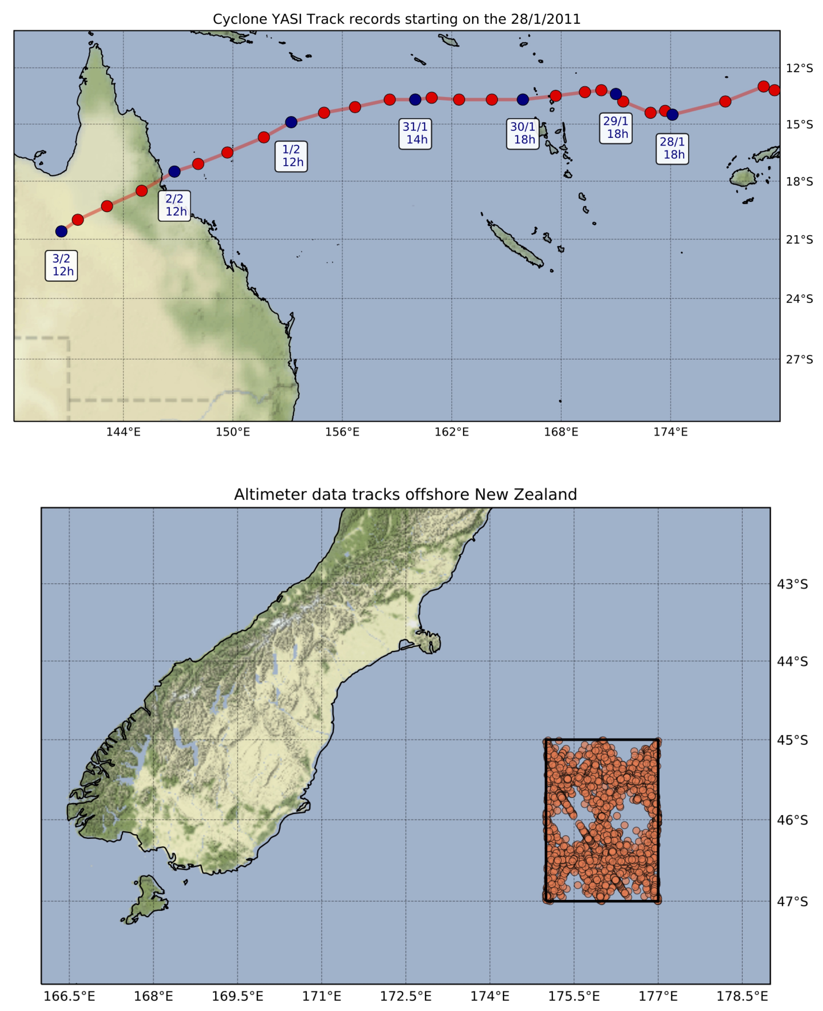
wa.plotCycloneTracks(title="Cyclone YASI Track", markersize=100, zoom=4,
                   extent=[138, 180, -30, -10], fsize=(12, 10))

wa.visualiseData(title="Altimeter data", extent=[138, 180, -30, -10.0],
                markersize=35, zoom=4, fsize=(12, 10), fsave=None)
plotTimeSeriessee the plotTimeSeries API for the available options.computeSeasonalCharacteristicssee the computeSeasonalCharacteristics API for the available options.
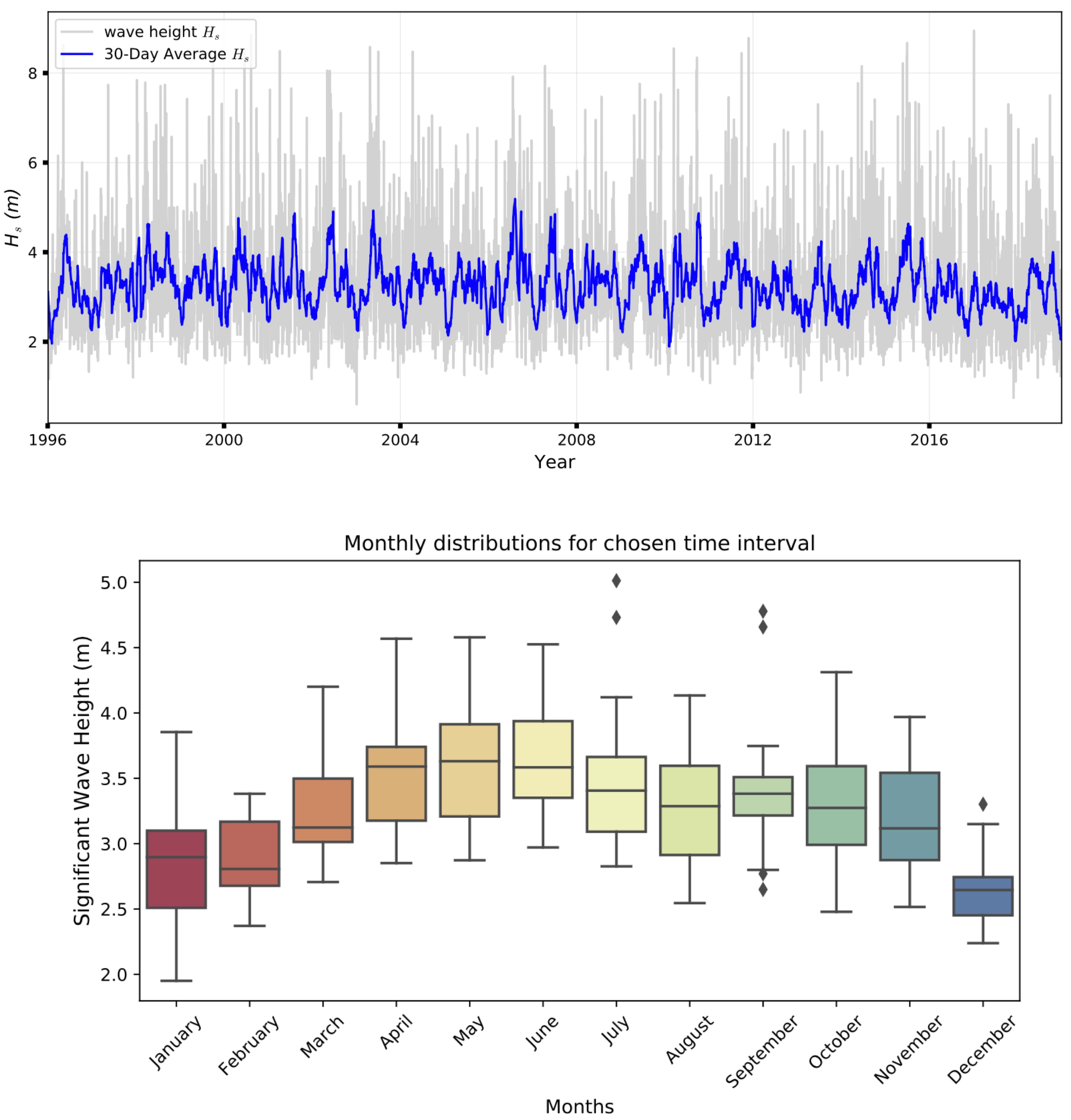
wa.plotTimeSeries(time=[1995,2016], series='H', fsize=(12, 5), fsave='seriesH')
whdata = wa.computeSeasonalCharacteristics(series='wh', time=[1998,2018], lonlat=None, fsave='whall', plot=True)
plotCycloneAltiPointsee the plotCycloneAltiPoint API for the available options.
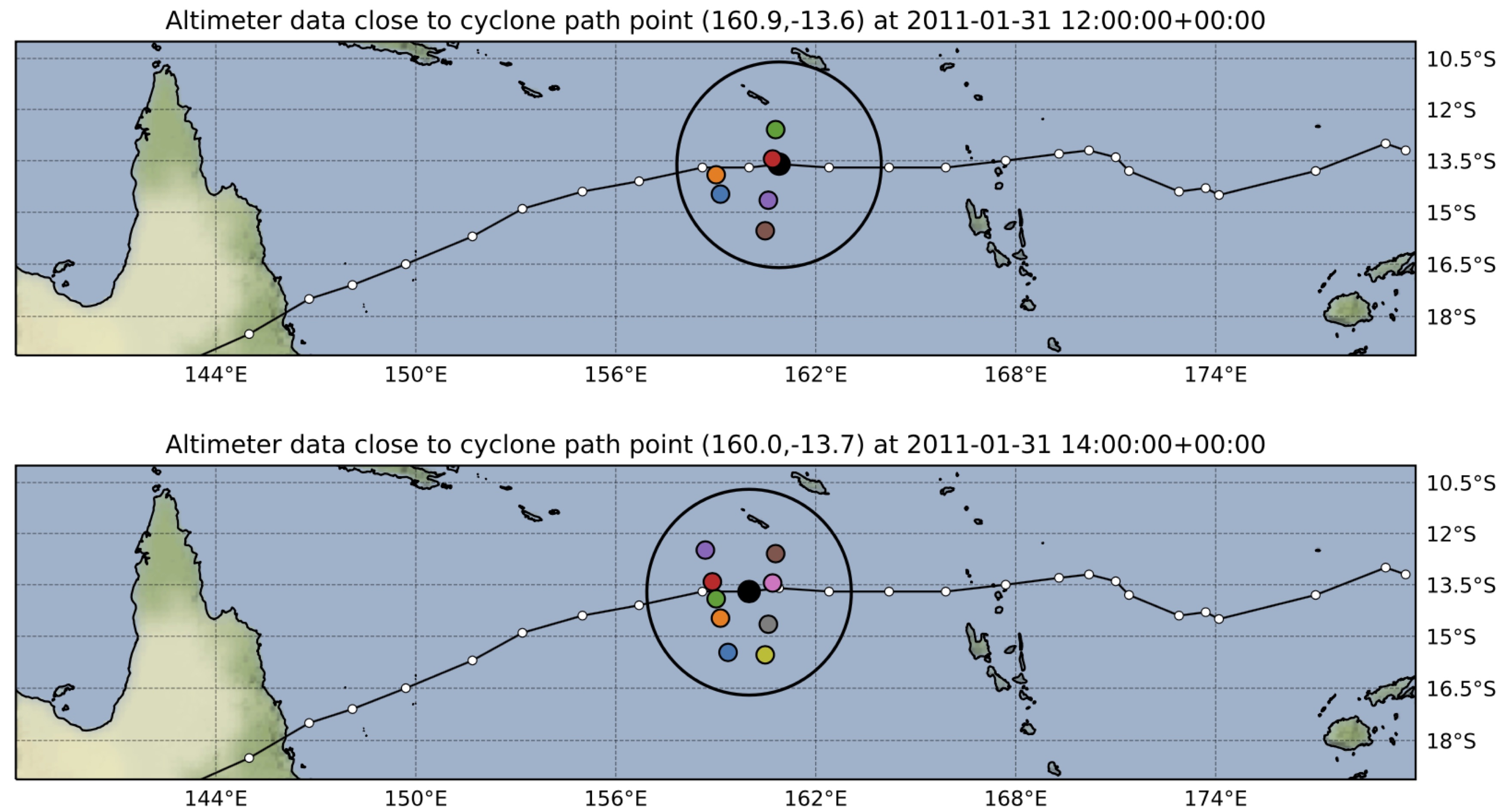
wa.plotCycloneAltiPoint(showinfo=True, extent=[138, 180, -18, -10],
                markersize=35, zoom=4, fsize=(12, 5))
Running examples
There are different ways of using the RADWave package. If you used a local install with pip, you can download the Jupyter Notebooks provided in the Github repository…
$ git clone https://github.com/pyReef-model/RADWave.git
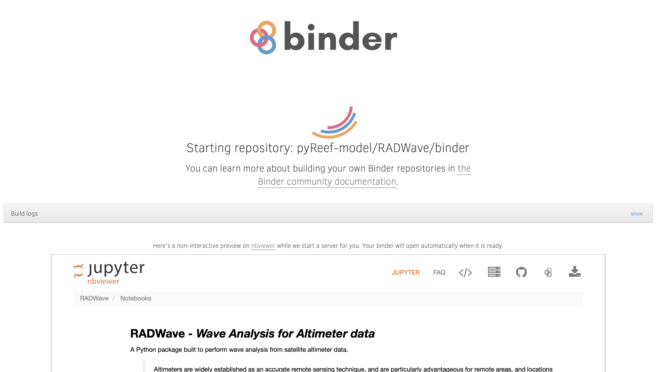
Binder
The series of Jupyter Notebooks can also be ran with Binder that opens those notebooks in an executable environment, making the package immediately reproducible without having to perform any installation.
This is by far the most simple method to test and try this package, just launch the demonstration at RADWave-live (mybinder.org)!
Docker
Another straightforward installation that again does not depend on specific compilers relies on the docker virtualisation system. Simply look for the following Docker container pyreefmodel/radwave.
Note
For non-Linux platforms, the use of Docker Desktop for Mac or Docker Desktop for Windows is recommended.
| [Ribal2019] | Ribal, A. & Young, I. R. - 33 years of globally calibrated wave height and wind speed data based on altimeter observations. Scientific Data 6(77), p.100, 2019. |